Top 5 Python Modules for Math You Wish You Knew Existed Earlier

Doing math has always involved performing numerical calculations. Sometimes, these calculations can become complex and tedious, and we may wish to ignore the numerical parts and only focus our brain power on the logical and inferential parts instead. This can save us a significant amount of time, and it is the main reason calculators were invented. The development of programmable computers has automated this process and made it easily accessible. Programming languages such as Python come with bundled packages called modules that can perform specific tasks, such as mathematics. Therefore, Python is not limited to just creating desktop applications and web development, but it can also be utilized for mathematical calculations. In this article, I will introduce 5 cool Python libraries that can be used to perform mathematical tasks. In case you are not familiar with the term "module", let me try to explain it in simple terms. Let's say I wrote a 7-line code that calculates the volume of a cylinder given its radius and length. I can then package this code so that it is reusable, and you don't need to write the code again; all you need is to call the function, and it will give you the result. In short, a module can define functions, classes, and variables, and it can also include runnable code. It is designed to help organize and reuse code and make it easy to import and use code from other modules. At the end I will guide you on how to install the modules in case you are not sure how to.

1. Matplotlib

At the top of the list is the Matplotlib module. Matplotlib is a plotting library that can be used to create a variety of plots, such as line plots, scatter plots, and histograms. It does not require extensive programming knowledge to be able to use it. All you need to do is define your x and y variables.

Below is a simple code that produces a line that passes through the given points.

import matplotlib.pyplot as plt

# Sample data
x = [1, 2, 3, 4, 5]
y = [2, 4, 6, 8, 10]

# Create a line plot
plt.plot(x, y)

# Add labels and title
plt.xlabel('X-axis')
plt.ylabel('Y-axis')
plt.title('Sample Line Plot')

# Display the plot
plt.show()

Now let's create a sine wave using the code below.

import numpy as np
import matplotlib.pyplot as plt

# Create a range of values for the x-axis
x = np.arange(0, 100, 0.001C

# Compute the y-values for a sine wave
y = np.sin(x)

# Create a plot of the sine wave
plt.plot(x, y)

# Add labels and a title to the plot
plt.xlabel('x')
plt.ylabel('y')
plt.title('Sine Wave')

# Display the plot
plt.show()

This is what I get when I run the code. My sine function has been plotted from 0 to 100 with 0.001 being the size between every x value being plotted. This is defined by the 4th line of the code. You can try to play around with different values. The more points you have i.e the less space between each point then the more smoother your sine wave will be.

Output:

To access the documentation for Matplotlib, you can visit the official Matplotlib website

2. SYMPY

SymPy is a Python library for symbolic mathematics. With SymPy, you can do things like symbolic mathematics, calculus, algebra, geometry, and more, all within Python. I have always enjoyed doing compass and straightedge geometry but analytic geometry is where I draw the line! (pun intended)

I mean bisecting angles is way more fun than plotting points. Rene Descartes would kill me for saying so:) SymPy has powerful tools for plotting functions and data in 2D and 3D, allowing you to visualize data sets. It also has a physics module that allows you to perform physics calculations, such as computing forces and moments, solving for equilibrium positions, and more. It extends to both differential and integral calculus. You can find the SymPy documentation on the project's website

3. Shapely

It is used to create and analyze 2D and 3D objects such as points, lines, polygons and many more.

Below is a code that plots a point, a line and a polygon. It then checks whether the point lies inside the polygon and also whether the line intersects it.

from shapely.geometry import Point, LineString, Polygon

# Create a Point object
point = Point(0.1, 0.1)

# Create a LineString object
line = LineString([(0.0, 0.0), (1.0, 1.0), (2.0, 1.5)])

# Create a Polygon object
polygon = Polygon([(0.0, 0.0), (0.0, 1.0), (1.0, 1.0), (1.0, 0.0)])

# Check if the point is inside the polygon
if point.within(polygon):
    print("The point is inside the polygon.")
else:
    print("The point is outside the polygon.")

# Check if the line intersects the polygon
if line.intersects(polygon):
    print("The line intersects the polygon.")
else:
    print("The line does not intersect the polygon.")

4. NetworkX

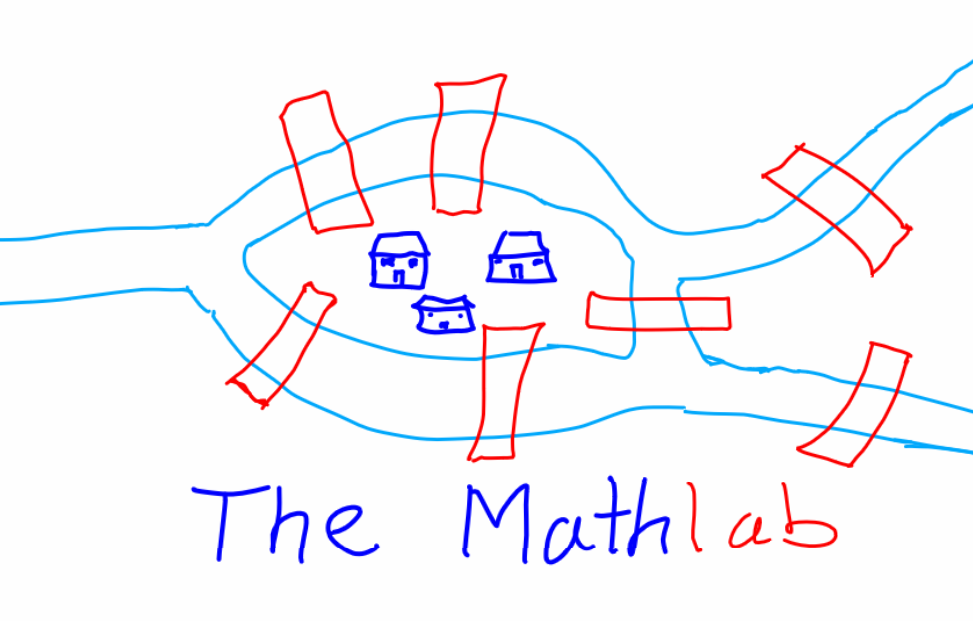
Are you even a math geek if you've never heard of the Königsberg bridge problem? This puzzle, first posed by Euler in the 18th century, is often used as an introductory story in most, if not all, graph theory textbooks. In fact, it is this puzzle that led to the development of graph theory itself. The Königsberg bridge problem asks whether it is possible to take a walk through the city of Königsberg, which was situated on both sides of the Pregel River and included two large islands connected to each other and the mainland by seven bridges, in such a way that you cross each of the seven bridges exactly once and return to your starting point. Below is an illustration of Königsberg with its 7 bridges:

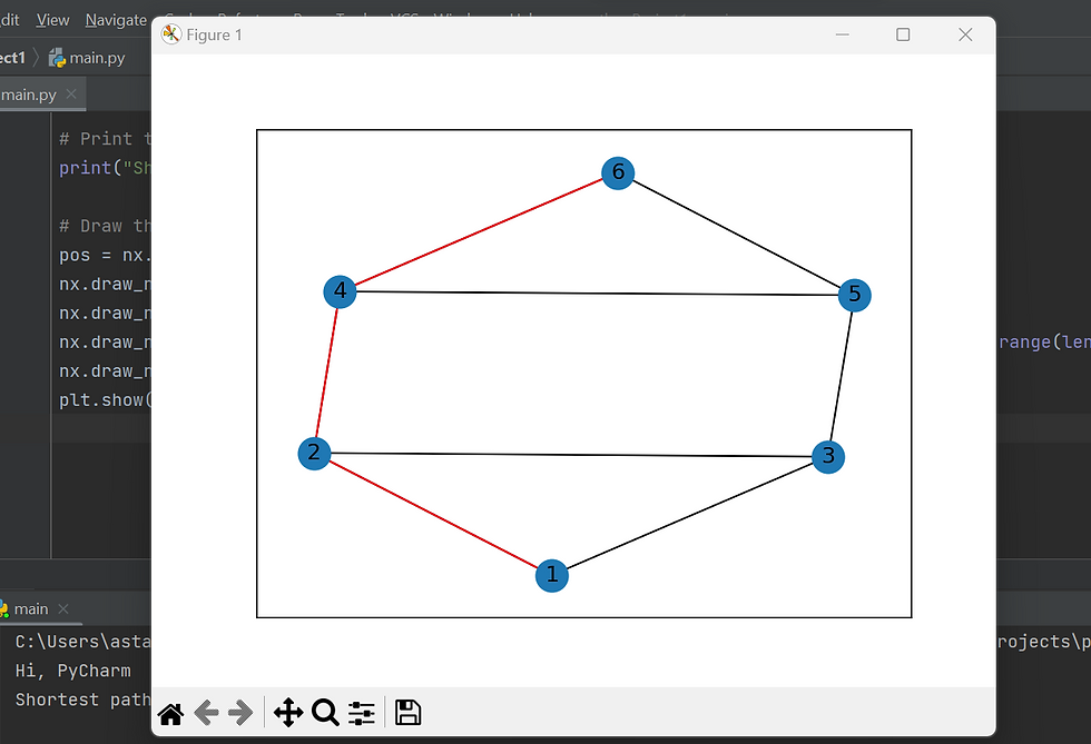
Euler used graph theory to prove that it is impossible if more than two of the vertices have an odd number of edges connected to them. Surprisingly, NetworkX was not available during Euler's time. Today, with NetworkX, you can easily study complex graphs with thousands of nodes and edges, and perform various graph algorithms such as centrality, clustering, shortest path, and more. NetworkX also offers powerful visualization tools to help you understand the structure and properties of your graphs. The code below plots 6 nodes with defined connection and then computes the shortest path from node 1 to 6

import networkx as nx
import matplotlib.pyplot as plt

# Create a graph
G = nx.Graph()
G.add_nodes_from([1, 2, 3, 4, 5, 6])
G.add_edges_from([(1, 2), (1, 3), (2, 3), (2, 4), (3, 5), (4, 5), (4, 6), (5, 6)])

# Find the shortest path between nodes 1 and 6
shortest_path = nx.shortest_path(G, source=1, target=6)

# Print the shortest path
print("Shortest path:", shortest_path)

# Draw the graph with the shortest path highlighted in red
pos = nx.spring_layout(G)
nx.draw_networkx_nodes(G, pos)
nx.draw_networkx_edges(G, pos)
nx.draw_networkx_edges(G, pos, edgelist=[(shortest_path[i], shortest_path[i+1]) for i in range(len(shortest_path)-1)], edge_color='r')
nx.draw_networkx_labels(G, pos)
plt.show()

Output:

Note that there are actually two shortest paths: [1, 3, 5, 6] and [1, 2, 4, 6]

You can find the documentation for NetworkX here

5. Pandas

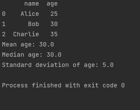
Pandas is a popular Python library for data manipulation and analysis. It supports a wide range of data formats, including CSV, Excel, SQL databases, and more. Here is a simple example of how to use Pandas to create a DataFrame, add data to it, and perform some basic operations.

import pandas as pd

# create a DataFrame with two columns, 'name' and 'age'
df = pd.DataFrame(columns=['name', 'age'])

# add data to the DataFrame
df.loc[0] = ['Alice', 25]
df.loc[1] = ['Bob', 30]
df.loc[2] = ['Charlie', 35]

# print the contents of the DataFrame
print(df)

# compute some basic statistics on the age column
print("Mean age:", df['age'].mean())
print("Median age:", df['age'].median())
print("Standard deviation of age:", df['age'].std())

Output:

The documentation for Pandas can be found here .

Guide on installing the modules

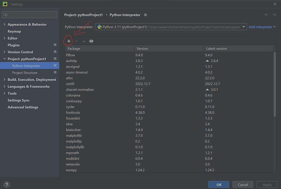
Installing your favourite Python module can't get any easier. If you are using the Pycharm IDE, then click on the file menu and go to the settings option on the drop down list. A window will appear then click on the + as shown below.

Then search for the name of the module you want to install and click the install package button at the bottom left section.

Once the installation is done all you have is to close the Pycharm application, reopen it again and you are ready to go!